This may seem a weird question for those that are not familiar with SFMC SQL Query Activities because they do not realize the crazy amount of different ways you can use different functions to accomplish the same end result table segmentation.
Now, just because the end result is identical, this does not mean that each process and path is identical. In fact, they are vastly different from each other. For the sake of time, I am going to concentrate on just the most popular ones:
- Rank and Total
- NTILE()
- _CustomObjectKey and MOD()
- TOP X with LEFT JOIN
- TOP X with NOT EXISTS
Now if by the above you don’t quite get what each one is, that is fine as I will be going into further detail below. I chose these 5 because they are the most popular choices and are the ones I think tend to be the most efficient and effective.
Speaking of effectiveness and efficiency, I want to start right off the bat that **there is no best solution** – it is all depending on context, preference and business requirements. Best practice and ‘best for me’ does not mean ‘best for you’. Anyone that says differently can go suck on a log.
Now you may ask, if I am not here to tell you what is the best or what you need to do to segment right, what am I doing? Well, my goal is to lay out each of the different options with all the pros/cons and other information I can to help you make the best educated decision for your own needs.
Rank and Total
Rank and Total is honestly my personal favorite and go to segmentation choice. The reason why is that this one is most definitely the most accurate and versatile methods to split your audience. To utilize this method, you would need to utilize the Rank() SQL function along with Count() inside a staging query to push this to a staging table. Then from that staging table, you would separate it out using math to find the percentages.
Rank() is basically a way to assign a corresponding row number (based on a partition if you want) to each record.
Count() is used to grab the total number of rows in the master data extension to pass along for reference on each record.
Rank and Total Staging
SELECT  Subscriberkey
      , EmailAddress
      , Field1 as Field1
      , Field2 as Field2
      , rank() over (ORDER BY newid()) as rn
      , oa.total as total
FROM [myMasterDE]
OUTER APPLY ( SELECT count(SubscriberKey) as total FROM [myMasterDE]) oa
/* Target: staging_table */
This query will add fields ‘rn’ and ‘total’ to a staging table where rn is the rank or numbering of each data row and total is the overall count of the master de. Through this you would then utilize some math to correctly segment out the data into segments.
Example Queries:
SELECT  Subscriberkey
      , EmailAddress
      , Field1 as Field1
      , Field2 as Field2
FROM [staging_table]
WHERE rn <= (total * .05)
/* Target: DE_1 */

SELECT  Subscriberkey
      , EmailAddress
      , Field1 as Field1
      , Field2 as Field2
FROM [staging_table]
WHERE rn between (total * .06) AND (total * .10)
/* Target: DE_2 */

...3-19...

SELECT  Subscriberkey
      , EmailAddress
      , Field1 as Field1
      , Field2 as Field2
FROM [staging_table]
WHERE rn > (total * .95)
/* Target: DE_20 */
PROS:
The major benefit to this is the intense level of accuracy and customization that is able to be had here even on smaller sample sizes. Since you completely control the math and the partition etc. For instance, you can do segmentation inside segmentation using this by adding other rank fields with different partitions, etc. You can also do different value segmentation instead of equal percentages. (e.g. rn between (total * .1) AND (total * .50) and rn between (total * .05) AND (total * .1) that allows you to have a 40% split and a 5% split on the same staging table.
CONS:
The main issue that this method has is that it can be a heavier process then the others due to the setup and math involved. This can lead to timing out or other similar issues. Which means you are more likely to have to break these out into multiple queries to accomplish what other methods might be able to do in a single query. This also requires a staging table to be effective, which adds extra processing through added sql queries and data extensions.
NTILE
I personally have an aversion to NTILE(), but it is a very viable and heavily used segmentation method. NTILE is a windowing function that is powerful, but its name is not exactly easily translate to what it does – which is why usually you do not know to use it unless someone teaches or mentions it to you.
NTILE basically will assign out a number within a range you set (e.g. 1-20 – NTILE(20)) in buckets allowing you to set a flag for segmentation. You would first push the data with the NTILE flag to a staging query where you would then utilize these flags to separate out into the correct segmented data extensions.
NTILE Staging
SELECT  Subscriberkey
      , EmailAddress
      , Field1
      , Field2
      , NTILE(8) OVER(order by newid()) as [group]
FROM [myMasterDE]
/* Target: staging_table */
Now that we have the 8 different flags in our staging table, we just need to write out the below types of queries to gather the segments into each different segment:
SELECT  Subscriberkey
      , EmailAddress
      , Field1
      , Field2
FROM [staging_table]
WHERE group = 1
/* Target: DE_1 */

...2-7...

SELECT  Subscriberkey
      , EmailAddress
      , Field1
      , Field2
FROM [staging_table]
WHERE group = 8
/* Target: DE_8 */
PROS:
NTILE is by far one of the easiest methods to implement and is actually one of the most performant methods at lower volume and simpler complexity (see my sample run times below). It is a very solid and easy to understand and manipulate method. For instance, if you want to have differing percentages, you can do something like ntile(20) and then do WHERE group IN (1,2,3,4,5) (for 25%) and then WHERE group IN (6,7,8,9,10,11,12,13,14,15) (for 50%).
CONS:
NTILE works in buckets and the lower the sample size and the higher the NTILE max size, the less accurate it gets. For instance if you have NTILE(3) and 10 records, you would have four 1 records, three 2 records and three 3 records – making an uneven split and breaking your even percentages. NTILE also exponentially gets less efficient and perfomant the higher the volume becomes. This also requires a staging table to be effective, which adds extra processing through added sql queries and data extensions.
_CustomObjectKey and MOD()
This is an interesting one that is very fast and performant and is only possible inside of SFMC. Before I get too far into explaining this, I feel like I need to first dig into what is a ‘_CustomObjectKey’ as there is no official documentation on exactly what it is. The best place I have seen an explaination of _CustomObjectKey is in this note at the bottom of this page inside the Ampscript.guide and this Salesforce Stack Exchange Answer.
Basically, the _CustomObjectKey is a number identifier that is automatically added to each record added into a data extension. The field is hidden so you, as a user cannot view it through the UI or normal methods. This field is still available though, to those who know to use it, for usage in queries, etc.
Now we know the gist of _CustomObjectKey, but how does MOD() relate to it? Well, MOD or Modulus basically divides two values and the result is the remainder of the division. So for instance if you do 10 modulus 3, your return would be 1. (e.g. 10 % 3 = 1).
By utilizing the _CustomObjectKey as the numerator and the number of segments you want as the denominator, you can segment out your records into groups. Let’s say you have 8 groups you want to divide, you would use _customobjectkey % 8 and then have to have it equal to 0-7 as if it evenly divides into 8, it will be 0. Basically running on a 0 index compared to a 1 index as other functions like NTILE use.
Example Queries
SELECT  Subscriberkey
      , EmailAddress
      , Field1
      , Field2
FROM [myMasterDE]
WHERE _customobjectKey % 20 = 0

... 1-18 ...

SELECT  Subscriberkey
      , EmailAddress
      , Field1
      , Field2
FROM [myMasterDE]
WHERE _customobjectKey % 20 = 19
PROS:
The _CustomObjectKey field is indexed automatically and most logic utilizing it is actually very fast. This can help greatly for significant volumes to keep it under the 30 minute time out. It is also pretty simple and does not require a staging table to run off of, reducing the number of necessary SQL Queries, helping make it more performant.
CONS:
_CustomObjectKey, although said to be auto-incrementing and sequential (I have heard from others this is not true so I would take this as a maybe not a guarantee), it can easily become convoluted and disparate from the number of records in the DE. For instance, when you overwrite data in the data extension, it will treat all of those records as ‘new’ records and renumber them. This makes the accuracy of using this method questionable as there is a lot of unknowns around it and it is dependent on these numbers being sequential. This also can run into accuracy issues like NTILE depending on the size of the audience and the complexity and size of the segmentation logic.
_Top X With Left Joins
This method uses very simple logic and basic functions of SQL. It combines an explicit set TOP in the select statement along with a Left Join Exclusion. Very simple and very repeatable.
TOP is used to limit the returned rows in your SELECT query to a certain amount. In this case, it is used to correctly split into the percentages you want it to be separated into.
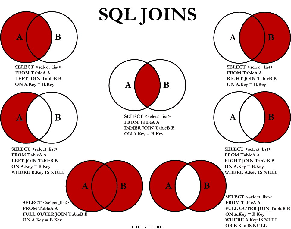
LEFT JOIN is used to connect a separate relational data extension to your current rowset to allow for reference and utilization of that data. To do a LEFT JOIN EXCLUSION you would do the left join and follow it with a WHERE statement saying that the primary key/foreign key on the joined DE is null.
Example Left Join Exclusion:
SELECT a.Subkey,
  b.Number
FROM [de1] a
LEFT JOIN [de2] b ON a.Subkey = b.Subkey
WHERE b.Subkey IS NULL
The above would return all records in de1 that do not exist in de2. Pretty neat, right?
To help share a cool graphic that has saved my butt a million times, here is a great visualization on SQL Joins:
Now that we have the way that the Joins work along with what TOP is, let’s take a look at how this method works:
Example Queries
SELECT  TOP 20000
        d.Subscriberkey
      , d.EmailAddress
      , d.Field1
      , d.Field2
from myMasterDE as d
order by newID()
/* target: DE_1 */


SELECT  TOP 20000
        d.Subscriberkey
      , d.EmailAddress
      , d.Field1
      , d.Field2
from myMasterDE as d
left join DE_1 d1 on (d1.SubscriberKey = d.SubscriberKey)
where d1.SubscriberKey is null
order by newID()
/* target: DE_2 */


SELECT  TOP 20000
        d.Subscriberkey
      , d.EmailAddress
      , d.Field1
      , d.Field2
from myMasterDE as d
left join DE_1 d1 on (d1.SubscriberKey = d.SubscriberKey)
left join DE_2 d2 on (d2.SubscriberKey = d.SubscriberKey)
where d1.SubscriberKey is null
where d2.SubscriberKey is null
order by newID()
/* target: DE_3 */


... 4-19 ...


SELECT  TOP 20000
        d.Subscriberkey
      , d.EmailAddress
      , d.Field1
      , d.Field2
from myMasterDE as d
left join DE_1 d1 on (d1.SubscriberKey = d.SubscriberKey)
left join DE_2 d2 on (d2.SubscriberKey = d.SubscriberKey)
left join DE_3 d3 on (d3.SubscriberKey = d.SubscriberKey)
left join DE_4 d4 on (d4.SubscriberKey = d.SubscriberKey)
left join DE_5 d5 on (d5.SubscriberKey = d.SubscriberKey)
left join DE_6 d6 on (d6.SubscriberKey = d.SubscriberKey)
left join DE_7 d7 on (d7.SubscriberKey = d.SubscriberKey)
left join DE_8 d8 on (d8.SubscriberKey = d.SubscriberKey)
left join DE_9 d9 on (d9.SubscriberKey = d.SubscriberKey)
left join DE_10 d10 on (d10.SubscriberKey = d.SubscriberKey)
left join DE_11 d11 on (d11.SubscriberKey = d.SubscriberKey)
left join DE_12 d12 on (d12.SubscriberKey = d.SubscriberKey)
left join DE_13 d13 on (d13.SubscriberKey = d.SubscriberKey)
left join DE_14 d14 on (d14.SubscriberKey = d.SubscriberKey)
left join DE_15 d15 on (d15.SubscriberKey = d.SubscriberKey)
left join DE_16 d16 on (d16.SubscriberKey = d.SubscriberKey)
left join DE_17 d17 on (d17.SubscriberKey = d.SubscriberKey)
left join DE_18 d18 on (d18.SubscriberKey = d.SubscriberKey)
left join DE_19 d19 on (d19.SubscriberKey = d.SubscriberKey)
where d1.SubscriberKey is null
and d2.SubscriberKey is null
and d3.SubscriberKey is null
and d4.SubscriberKey is null
and d5.SubscriberKey is null
and d6.SubscriberKey is null
and d7.SubscriberKey is null
and d8.SubscriberKey is null
and d9.SubscriberKey is null
and d10.SubscriberKey is null
and d11.SubscriberKey is null
and d12.SubscriberKey is null
and d13.SubscriberKey is null
and d14.SubscriberKey is null
and d15.SubscriberKey is null
and d16.SubscriberKey is null
and d17.SubscriberKey is null
and d18.SubscriberKey is null
and d19.SubscriberKey is null
order by newID()
/* target: DE_20 */
PROS:
It is fairly simple to read and to replicate/edit even without strong SQL skills. Logic is easy to see and edit inside the query to help exclude all those that were already segmented out.
CONS:
The more complex it gets or the more segments, the more unwieldy that this method gets. See above example for DE_20. It also is not super performant so can potentially lead to timeouts, especially at larger volumes and complexities. You will also need to do math beforehand to get the exact number for the ‘TOP’ declaration for your segments. Also due to the repetitive nature, some maintenance may be arduous as you would need to do the change in multiple places across multiple queries – increasing risk of human error or mistakes.
_Top X With Not Exists
This method is extremely similar to Top X with Left Join Exclusions. But, instead of excluding using Left Joins, you exclude using the Not Exists() function. To sum things up, Exists(), which is the actual function, will look at a subquery encased inside of the parenthesis in the function and verify if the current record exists in that subquery results.
The Not before it basically flips the return of the function. So if it would return TRUE stating that it does exist in the function, it would instead return FALSE and vice versa. Why would we want that? Well, each WHERE statement or condition will only continue down the path if (within the operators) it returns a TRUE result.
We want it to exclude those that do exist in that subquery, so we want the ‘pass’ aka TRUE (that it exists in there) to become the ‘fail’ or FALSE, so we achieve that by placing NOT in front of the function.
So basically in this we would be replacing the Left Join and the conditional where statement at the end of the query and replacing it with a WHERE NOT EXISTS() condition.
Example Not Exists Exclusion:
SELECT a.Subkey,
  b.Number
FROM [de1] a
WHERE NOT EXISTS(SELECT TOP 1 ex.Subkey FROM [de2] ex WHERE a.Subkey = ex.Subkey)
The above would return all records in de1 that do not exist in de2. In my opinion this version is much neater and easier to manage/understand than Left Join, but to each their own.
You may notice that in the NOT EXISTS() subquery I am using TOP 1. The reason I am using this is to limit the return to reduce processing. By having the condition inside the subquery be a match of the primary keys on both tables, we only need 1 result to prove true/false.
Now that we know how the Not Exists part works in this method, let’s take a look at how this method works:
Example Queries
select top 125000
d.SubscriberKey
, d.emailAddress
, d.Field1
, d.Field2
from myMasterDE as d
order by newID()
/* target: DE_1 */


select top 125000
d.SubscriberKey
, d.emailAddress
, d.Field1
, d.Field2
from myMasterDE as d
where NOT EXISTS(SELECT TOP 1 ex.SubscriberKey FROM [DE_1] ex WHERE ex.SubscriberKey = d.SubscriberKey)
order by newID()
/* target: DE_2 */


select top 125000
d.SubscriberKey
, d.emailAddress
, d.Field1
, d.Field2
from myMasterDE as d
where NOT EXISTS(SELECT TOP 1 ex.SubscriberKey FROM [DE_1] ex WHERE ex.SubscriberKey = d.SubscriberKey)
where NOT EXISTS(SELECT TOP 1 ex.SubscriberKey FROM [DE_2] ex WHERE ex.SubscriberKey = d.SubscriberKey)
order by newID()
/* target: DE_3 */


...4-19...


select top 125000
d.SubscriberKey
, d.emailAddress
, d.Field1
, d.Field2
from myMasterDE as d
where NOT EXISTS(SELECT TOP 1 ex.SubscriberKey FROM [DE_1] ex WHERE ex.SubscriberKey = d.SubscriberKey)
where NOT EXISTS(SELECT TOP 1 ex.SubscriberKey FROM [DE_2] ex WHERE ex.SubscriberKey = d.SubscriberKey)
where NOT EXISTS(SELECT TOP 1 ex.SubscriberKey FROM [DE_3] ex WHERE ex.SubscriberKey = d.SubscriberKey)
where NOT EXISTS(SELECT TOP 1 ex.SubscriberKey FROM [DE_4] ex WHERE ex.SubscriberKey = d.SubscriberKey)
where NOT EXISTS(SELECT TOP 1 ex.SubscriberKey FROM [DE_5] ex WHERE ex.SubscriberKey = d.SubscriberKey)
where NOT EXISTS(SELECT TOP 1 ex.SubscriberKey FROM [DE_6] ex WHERE ex.SubscriberKey = d.SubscriberKey)
where NOT EXISTS(SELECT TOP 1 ex.SubscriberKey FROM [DE_7] ex WHERE ex.SubscriberKey = d.SubscriberKey)
where NOT EXISTS(SELECT TOP 1 ex.SubscriberKey FROM [DE_8] ex WHERE ex.SubscriberKey = d.SubscriberKey)
where NOT EXISTS(SELECT TOP 1 ex.SubscriberKey FROM [DE_9] ex WHERE ex.SubscriberKey = d.SubscriberKey)
where NOT EXISTS(SELECT TOP 1 ex.SubscriberKey FROM [DE_10] ex WHERE ex.SubscriberKey = d.SubscriberKey)
where NOT EXISTS(SELECT TOP 1 ex.SubscriberKey FROM [DE_11] ex WHERE ex.SubscriberKey = d.SubscriberKey)
where NOT EXISTS(SELECT TOP 1 ex.SubscriberKey FROM [DE_12] ex WHERE ex.SubscriberKey = d.SubscriberKey)
where NOT EXISTS(SELECT TOP 1 ex.SubscriberKey FROM [DE_13] ex WHERE ex.SubscriberKey = d.SubscriberKey)
where NOT EXISTS(SELECT TOP 1 ex.SubscriberKey FROM [DE_14] ex WHERE ex.SubscriberKey = d.SubscriberKey)
where NOT EXISTS(SELECT TOP 1 ex.SubscriberKey FROM [DE_15] ex WHERE ex.SubscriberKey = d.SubscriberKey)
where NOT EXISTS(SELECT TOP 1 ex.SubscriberKey FROM [DE_16] ex WHERE ex.SubscriberKey = d.SubscriberKey)
where NOT EXISTS(SELECT TOP 1 ex.SubscriberKey FROM [DE_17] ex WHERE ex.SubscriberKey = d.SubscriberKey)
where NOT EXISTS(SELECT TOP 1 ex.SubscriberKey FROM [DE_18] ex WHERE ex.SubscriberKey = d.SubscriberKey)
where NOT EXISTS(SELECT TOP 1 ex.SubscriberKey FROM [DE_19] ex WHERE ex.SubscriberKey = d.SubscriberKey)
order by newID()
/* target: DE_3 */
PROS:
It is easy to understand and each exclusion is pretty much self contained so its harder to miss maintenance or edits. By using something that shows the context of it being an exclusion (NOT EXISTS) it is easier for those that may be less technical or well versed in SQL to understand what it is doing.
CONS:
As with the Left Join Exclusion, this gets more and more unwieldy as it gets more complex. It also has similar performance rates as the Left Join so it can fall over on high volumes as well. This also requires the math beforehand to get the correct numbers to fill in for TOP to define your segments. Also, although less so then with the Left Join Exclusion, it is fairly repetitive code, so it opens the possibility of human error/mistakes when maintaining or editing.
So, What does this mean?
Although the above info is very useful, I am sure you are reading through (thanks for reading!) going ‘Hey! When is he going to tell us which one is the best?’ Sadly, there is no ultimate best solution for this – it is very contextual! Now, I know this can sound like a cop-out, so I am going to share some info I got from performance tests as well as my recommendations on a few scenarios. Hopefully this will help get you on the right path to figuring out which is the right method for you.
Performance Tests
Below are a few performance test averages I ran across a few different BU environments at different times to try and get as accurate numbers as I could. I ran these with each record only having 4 columns of information and very little logic outside the segmentation involved. This is not to be used as a guideline for how long your queries will run, but more as a comparison of how efficient each one was in the run/test.
100,000 records | 5 groups – Automated
For this run, I had a master data extension that everything was pulled from that held 100,000 records in it. The segmentation was into 5 equal audiences.
| Group | Time |
|---|---|
| rank/total | 7:08 |
| ntile | 4:30 |
| _customObjectKey | 6:18 |
| topJoin | 6:21 |
| topNotExists | 6:22 |
As you can see from this result, the most performant by far was NTILE. This ran at average 70% of the runtime of the others. This is impressive especially considering that it requires a staging table, so it needs an extra query and data extension to run.
Another thing to note is that _customObjectKey ran almost in parallel with the Top Join and Top Not Exists queries, despite that it is supposed to be far superior in processing requirements/speed.
1,000,000 records | 8 groups – Automated
For this run, I had a master data extension that everything was pulled from that held 1,000,000 records in it. The segmentation was into 8 equal audiences. This was to test out at higher volume and complexity and validate efficiencies beyond the smaller audience.
| Group | Time |
|---|---|
| rank/total | 17:34 |
| ntile | 17:37 |
| _customObjectKey | 16:52 |
| topJoin | 17:18 |
| topNotExists | 17:26 |
As you can see, very different results than what you saw in the previous test. NTILE went from by far the superior method to the worst run time of the bunch. Also, CustomObjectKey has started to shine through with its superior performance, but as you notice it is only minimal improvements, not enough to truly declare it as the highest performer.
You will also notice that the Rank and Total numbers are actually fairly in line with the other methods, making this a much more viable method for larger audiences. It even outperformed NTILE.
My Conclusions
So, I do want to note that above tests are not concrete or conclusive, they are just what I have gathered in a few different contexts running through different times and stacks. My conclusions are based on these numbers as well as my knowledge and expertise of SQL.
For high volume queries with multiple groupings, I would highly recommend the Rank and Total as your preferred method due to the flexibility and accuracy as well that the runtime is not significantly higher. If this is not an option, my second recommendation would be CustomObjectKey as its simplistic and ran the fastest, so its performant. I just have the worry on the accuracy of the segmentation, which is why I move this to second.
For low volume queries with limited groupings, I would recommend NTILE() as its mostly accurate and ran at a significantly faster rate than any of the other methods. This seemed to be the highest performer by far. The only caveat is if you are having low volume with complex groupings, then you may want to explore the Rank and Total to ensure your margin of error is as small as possible.
Although I did not choose either of the ‘Top’ methods as my optimal recommendations, that does not mean they are not potentially the best option for your scenario – I know many highly skilled and experienced SFMC users that use those as their ‘go to’ segmentation method.